Graph compression#
The compression pipeline is implemented on top of the WebGraph framework. It takes an ORC Graph Dataset as an input, such as the ones found in the Graph Dataset List, and generates a compressed graph suitable for high intensity analyses on large servers.
Running the compression pipeline#
Dependencies#
To compress a graph, you will need to install the swh.graph tool as well as
a recent JRE, as described in the Quickstart page.
You will also need the zstd compression tool:
$ sudo apt install zstd
Hardware Requirements#
The compression pipeline is even more demanding than the graph server in terms of hardware requirements, especially RAM. Notably, the BFS compression step loads a graph compressed in random order in memory, which is usually more than a TiB for the full graph. While it is possible to do this step with a memory mapping, our experiments show that this could take a very long time (several months) on hard drives.
The LLP compression step requires 13 bytes of RAM per node, which could amount to storing hundreds of gigabytes in RAM in addition to loading the graph itself.
Some steps also involve sorting the entire set of edges and their labels, by using large on-disk buffer files, sometimes reaching the size of the input data itself.
The machine we used to compress the entire graph (dataset version 2024-12-06) is a HPE ProLiant DL380 Gen10 Plus with the following hardware specs:
4 TiB of RAM (30 × DDR4 LRDIMM 128 Go )
2 CPUs with 48 threads each (Intel Xeon Gold 6342 CPU @ 2.80GHz)
77 TiB of SSD (NVMe)
Input dataset#
First, you need to retrieve a graph to compress, in ORC format. The Graph Dataset List has a list of datasets made available by the Software Heritage archive, including “teaser” subdatasets which have a more manageable size and are thus very useful for prototyping with less hardware resources.
The datasets can be retrieved from S3 or the annex, in a similar fashion to what is described in Retrieving a compressed graph, by simply replacing “compressed” by “orc”:
(venv) $ mkdir -p 2021-03-23-popular-3k-python/orc
(venv) $ cd 2021-03-23-popular-3k-python/
(venv) $ aws s3 cp --no-sign-request --recursive s3://softwareheritage/graph/2021-03-23-popular-3k-python/orc/ orc
Alternatively, any custom ORC dataset can be used as long as it respects the schema of the Software Heritage Graph Dataset.
Note: for testing purposes, a fake test dataset is available in the
swh-graph repository, with just a few dozen nodes. The ORC tables are
available in swh-graph/swh/graph/example_dataset/orc/.
Compression#
You can compress your dataset by using the swh graph compress command. It
will run all the various steps of the pipeline in the right order.
(venv) $ swh graph compress --input-dataset orc/ --output-directory compressed/
[...]
(venv) $ ls compressed/
graph.edges.count.txt
graph.edges.stats.txt
graph.graph
graph.indegree
graph-labelled.labeloffsets
graph-labelled.labels
[...]
graph-transposed.obl
graph-transposed.offsets
graph-transposed.properties
(The purpose of each of these files is detailed in the Rust API tutorial.)
For sufficiently large graphs, this command can take entire weeks. It is highly recommended to run it in a systemd service or in a tmux session.
It is also possible to run single steps or step ranges from the CLI:
swh graph compress -i orc/ -o compressed/ --steps mph-bfs
See swh graph compress --help for syntax and usage details.
For some steps, we will need to open many files, so you should increase the limit if possible:
ulimit -Sn 1048576
Compression steps#
The compression pipeline consists of the following steps:
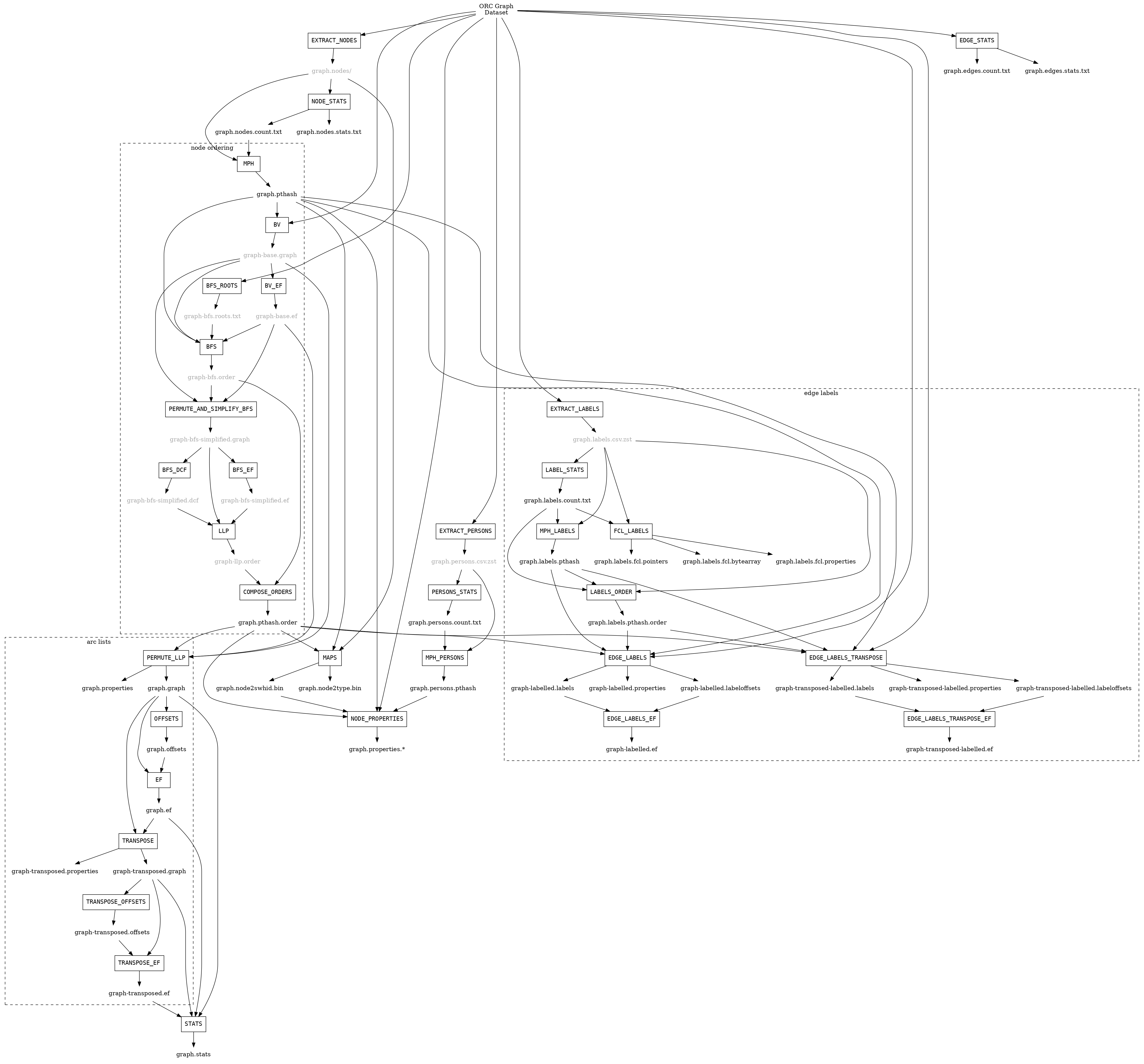
Compression steps#
Each of these steps is briefly described below. For more details see the original Software Heritage graph compression paper [SWHGraphCompression2020], as well as chapters 9 and 10 of Antoine Pietri’s PhD thesis [PietriThesis2021].
EXTRACT_NODES#
This step reads a graph dataset and extract all the unique node SWHIDs it contains, including the ones that are not stored as actual objects in the graph, but only referred to by the edges.
Rationale: Because the graph can contain holes, loose objects and dangling objects, some nodes that are referred to as destinations in the edge relationships might not actually be stored in the graph itself. However, to compress the graph using a graph compressio library, it is necessary to have a list of all the nodes in the graph, including the ones that are simply referred to by the edges but not actually stored as concrete objects.
This step reads the entire graph dataset, and uses sort -u to extract the
set of all the unique nodes and unique labels that will be needed as an input
for the compression process. It also write object count statistics in various
files:
The set of nodes is written in
graph.nodes/*.csv.zst, as a zst-compressed sorted list of SWHIDs, one per line, sharded into multiple files.
EXTRACT_LABELS#
This step works similarly to EXTRACT_NODES, but instead of extracting node SWHIDs, it extracts the set of all unique edge labels in the graph.
The set of edge labels is written in
graph.labels.csv.zst, as a zst-compressed sorted list of labels encoded in base64, one per line.
NODE_STATS / EDGE_STATS / LABEL_STATS#
NODE_STATS and LABEL_STATS read the list of unique SWHIDs and labels produced by EXTRACT_NODES and EXTRACT_LABELS. EDGE_STATS reads the ORC files themselves.
They then produce the total number of nodes/edges/labels, as well as the number of nodes and edges of each type.
The number of unique nodes referred to in the graph is written in a text file,
graph.nodes.count.txtThe number of unique edges referred to in the graph is written in a text file,
graph.edges.count.txtThe number of unique edge labels is written in a text file,
graph.labels.count.txtStatistics on the number of nodes of each type are written in a text file,
graph.nodes.stats.txtStatistics on the number of edges of each type are written in a text file,
graph.edges.stats.txt
MPH#
As discussed in the Rust API tutorial.) , a node in the Software Heritage data model is identified by its SWHID (see persistent identifiers), but WebGraph internally uses integers to refer to node ids.
To create a mapping between integer node IDs and SWHIDs, we use the pthash::PartitionedPhf<Minimal, MurmurHash2_128, DictionaryDictionary> structure, which (like any Minimal Perfect Hash function) maps N keys to N consecutive integers.
We run this function on the list of SWHIDs stored in the
graph.nodes/*.csv.zst file generated in the previous step.
This allows us to generate a bijection from the set of all the n SWHIDs in the
graph to the set of integers \([0, n - 1]\).
The step produces a graph.pthash file, containing a function which takes a SWHID
(as a bytestring) and returns its associated node ID.
Note
Graphs produced before 2024-08-20 has a graph.mph, which is a (Java-specific)
serialization of the
GOVMinimalPerfectHashFunction
class of the Sux4J library, instead of graph.pthash,
as well as a graph.cmph which is a portable representation of the same data.
Initial order#
This step is optional, but significantly improves memory requirement of the next step.
The MPH step causes nodes to be in a random order. A random order on nodes causes the graph produced by BV compress step to be very big, to the point it takes 3.6TB for the 2025-10-08 graph. This is a major issue for performance, because most of that graph needs to fit in memory for the BFS / BFS_ROOTS step, otherwise its runtime can be goes from days to weeks.
This optional step works around the issue by replacing the random order of the MPH step with an order constructed from a graph that was already compressed months ago. All nodes present in the current graph but not in the older graph are still in a random order, but they are a minority.
If enabled, this step produces its result in:
graph-base.order
BV compress#
This is the first actual compression step, where we build a compressed version of the input graph dataset.
This works by iterating through arcs in the ORC Graph dataset, turning it into
pairs of integers using the MPH obtained at the previous step,
then sorting them in an aggressively parallel fashion, then stores them as .bitstream files.
These .bitstream are then opened again by BatchIterator, then
merged
into an an ArcListGraph <https://docs.rs/webgraph/latest/webgraph/graphs/arc_list_graph/struct.ArcListGraph.html>.
This ArcListGraph is then read by BvComp which compresses it as a BVGraph, using the compression techniques described in the article The WebGraph Framework I: Compression Techniques cited above.
The resulting BV graph is stored as a set of files:
graph-base.graph: the compressed graph in the BV formatgraph-base.properties: entries used to correctly decode graph and offset files
BV_EF#
These steps produce the following file, which allows random access in the graph:
graph-base.ef: offsets values to read the bit stream graph file, compressed using an Elias-Fano representation and encoded with epserde <https://docs.rs/epserde/>.
BFS / BFS_ROOTS#
In [LLP], the paper authors empirically demonstrate that a high graph compression ratio can be achieved for the graph of the Web by ordering nodes such that vertices from the same host are close to each other.
In Software Heritage, there is no notion of “host” that can be used to generate these compression-friendly orderings, because the identifiers are just uniformly random cryptographic hashes. However, we can generate these orderings by running algorithms to inform us on which nodes are close to each other.
In this step, we run a BFS traversal on the entire graph to get a more compression-friendly ordering of nodes. We use the BFS class from the LAW library.
As an extra optimization, we make the BFS traversal start from origin nodes,
sorted by their URL after splitting it on / and reversing the order of components
to cluster similar projects/forks together.
This list is stored in graph-bfs.roots.txt
The resulting ordering is stored in a graph-bfs.order file, which contains
all the node IDs in the order of traversal.
PERMUTE_AND_SIMPLIFY_BFS / BFS_EF / BFS_DCF#
Once the BFS order is computed, we permute the initial “base” graph using the this new ordering and add the reverse of every arc.
The BFS-compressed graph is stored in the files:
graph-bfs.graphgraph-bfs.properties
Note
In the Java implementation this was done in three steps (permute, transpose, simplify) using the Transform class; but in the current Rust implementation we do all three at once, saving time by avoiding two BV compressions.
The BFS_EF and BFS_DCF steps then produce the following files:
graph-bfs.ef: offsets to allow random-access to the graphgraph-bfs.dcf: degree-cumulative function, to distribute load evenly in the next step
LLP#
Better compression ratios can be achieved by the Layered Label Propagation (LLP) algorithm to reorder nodes. This algorithm is described in [LLP]. The LLP algorithm finds locality-preserving orders by clustering together nodes in close proximity. Similar to the BFS, this algorithm is particularly interesting for our use case as it is unsupervised, and does not rely on prior information on the clusters present in the graph. The idea behind the clustering algorithm is to randomly distribute communities to the nodes in the graph, then iteratively assign to each node the community most represented in its neighbors.
Paolo Boldi, Marco Rosa, Massimo Santini, Sebastiano Vigna. Layered label propagation: a multiresolution coordinate-free ordering for compressing social networks. WWW 2011: 587-596 DOI: https://doi.org/10.1145/1963405.1963488 preprint: https://arxiv.org/abs/1011.5425
LLP is more costly than simple BFS-based compression in both time and memory. Even though the algorithm has a linear time complexity, it does multiple iterations on the graph and is significantly slower than the BFS which is just one single traversal. Moreover, keeping track of the communities requires a total of 13 bytes per node, which increases the RAM requirements. Because of these constraints, it is unrealistic to run the LLP algorithm on the uncompressed version of the graph; this is why we do an intermediate compression with the BFS ordering first, then compress the entire graph again with an even better ordering.
The LLP algorithm takes a simplified (loopless, symmetric) graph as an input, which we already computed in the previous steps.
The algorithm is also parameterized by a list of γ values, a “resolution” parameter which defines the shapes of the clustering it produces: either small, but denser pieces, or larger, but unavoidably sparser pieces. The algorithm then combines the different clusterings together to generate the output reordering. γ values are given to the algorithm in the form \(\frac{j}{2^k}\); by default, 12 different values of γ are used. However, the combination procedure is very slow, and using that many γ values could take several months in our case. We thus narrowed down a smaller set of γ values that empirically give good compression results, which are used by default in the pipeline. In general, smaller values of γ seem to generate better compression ratios. The effect of a given γ is that the density of the sparsest cluster is at least γ γ+1, so large γ values imply small, more dense clusters. It is reasonable to assume that since the graph is very sparse to start with, such clusters are not that useful.
The resulting ordering is stored in a graph-llp.order file.
PERMUTE_LLP / EF#
Once the LLP order is computed, we permute the BFS-compressed graph using the
this new ordering. The LLP-compressed graph, which is our final compressed
graph, is stored in the files graph.{graph,ef,properties}.
OBL#
Cache the BVGraph offsets of the forward graph to make loading faster. The
resulting offset big list is stored in the graph.obl file.
COMPOSE_ORDERS#
To be able to translate the initial MPH inputs to their resulting rank in the LLP-compressed graph, we need to use the two order permutations successively: the base → BFS permutation, then the BFS → LLP permutation.
To make this less wasteful, we compose the two permutations into a single
one. The resulting permutation is stored as a
graph.pthash.order file. Hashing a SWHID with the graph.pthash function, then
permuting the result using the graph.pthash.order permutation yields the integer
node ID matching the input SWHID in the graph.
Note
Graphs produced before 2024-08-20 have graph.mph and graph.order instead
of graph.pthash and graph.pthash.order.
TRANSPOSE / TRANSPOSE_EF#
Transpose the graph to allow backward traversal.
The resulting transposed graph is stored as the
graph-transposed.{graph,offsets,properties} files.
MAPS#
This steps generates the node mappings described in Node Types and SWHIDs. In particular, it generates:
graph.node2swhid.bin: a compact binary representation of all the SWHIDs in the graph, ordered by their rank in the graph file.graph.node2type.bin: a LongBigArrayBitVector which stores the type of each node.
It does so by reading all the SWHIDs in the graph.nodes.csv.zst file generated in the
EXTRACT_NODES step, then getting their corresponding node IDs (using the
.pthash and .pthash.order files), then sorting all the SWHIDs according to
their node ID. It then writes these SWHIDs in order, in a compact but seekable
binary format, which can be used to return the SWHID corresponding to any given
node in O(1).
EXTRACT_PERSONS#
This step reads the ORC graph dataset and extracts all the unique persons it contains. Here, “persons” are defined as the set of unique pairs of name + email, potentially pseudonymized, found either as revision authors, revision committers or release authors.
The ExtractPersons class reads all the persons from revision and release
tables, then uses sort -u to get a sorted list without any duplicates. The
resulting sorted list of authors is stored in the graph.persons/*.csv.zst
file.
MPH_PERSONS#
This step computes a Minimal Perfect Hash function on the set of all the unique
persons extracted in the EXTRACT_PERSONS step. Each individual person is mapped
to a unique integer in \([0, n-1]\) where n is the total number of
persons. The resulting function is serialized and stored in the
graph.persons.pthash file.
NODE_PROPERTIES#
This step generates the node property files, as described in Node Properties. The nodes in the Software Heritage Graph each have associated properties (e.g., commit timestamps, authors, messages, …). The values of these properties for each node in the graph are compressed and stored in files alongside the compressed graph.
The WriteNodeProperties class reads all the properties from the ORC Graph Dataset, then serializes each of them in a representation suitable for efficient random access (e.g., large binary arrays) and stores them on disk.
For persons (authors, committers etc), the MPH computed in the MPH_PERSONS step is used to store them as a single pseudonymized integer ID, which uniquely represents a full name + email.
The results are stored in the following list of files:
graph.property.author_id.bingraph.property.author_timestamp.bingraph.property.author_timestamp_offset.bingraph.property.committer_id.bingraph.property.committer_timestamp.bingraph.property.committer_timestamp_offset.bingraph.property.content.is_skipped.bits(formerly ingraph.property.content.is_skipped.binwhich was serialized in a Java-specific format)graph.property.content.length.bingraph.property.message.bingraph.property.message.offset.bingraph.property.tag_name.bingraph.property.tag_name.offset.bin
MPH_LABELS / LABELS_ORDER#
The MPH_LABELS step computes a Minimal Perfect Hash function on the set of all the unique arc label names extracted in the EXTRACT_LABELS step. Each individual arc label name (i.e., directory entry names and snapshot branch names) is mapped to a unique integer in \([0, n-1]\), where n is the total number of unique arc label names.
Then, LABELS_ORDER computes a permutation so these n values can be (uniquely) mapped to the position in the sorted list of labels.
The results are stored in:
graph.labels.pthashgraph.labels.pthash.order
Note
This step formerly computed a monotone Minimal Perfect Hash function on the set of all the unique arc label names extracted in the EXTRACT_NODES step. Each individual arc label name (i.e., directory entry names and snapshot branch names) is monotonely mapped to a unique integer in \([0, n-1]\), where n is the total number of unique arc label names, which corresponds to their lexical rank in the set of all arc labels.
In other words, that MPH being monotone meant that the hash of the k-th item in the sorted input list of arc labels will always be k. We use the LcpMonotoneMinimalPerfectHashFunction of Sux4J to generate this function.
The rationale for using a monotone function here is that it allowed us to
quickly get back the arc label from its hash without having to store an
additional permutation.
The resulting MPH function is serialized and stored in the graph.labels.mph
file.
As PTHash does not support monotone MPHs, we now compute a permutation in MPH_LABELS / LABELS_ORDER instead.
FCL_LABELS#
This step computes a reverse-mapping for arc labels, i.e., a way to efficiently get the arc label name from its hash computed with the MPH + permutation of the MPH_LABELS and LABELS_ORDER steps.
For this purpose, we use a reimplementation of the MappedFrontCodedStringBigList
class from the dsiutils library, using the graph.labels/*.csv.zst files as its
input. It stores the label names in a compact way by using front-coding
compression, which is particularly efficient here because the strings are
already in lexicographic order. The resulting FCL files are stored as
graph.labels.fcl.*, and they can be loaded using memory mapping.
EDGE_LABELS#
This step generates the edge property files, as described in Edge Labels. These files allow us to get the edge labels as we iterate on the edges of the graph. The files essentially contain compressed sorted triplets of the form (source, destination, label), with additional offsets to allow random access.
To generate these files, the LabelMapBuilder class starts by reading in parallel the labelled edges in the ORC dataset, which can be thought of as quadruplets containing the source SWHID, the destination SWHID, the label name and the entry permission if applicable:
swh:1:snp:4548a5… swh:1:rev:0d6834… cmVmcy9oZWFkcy9tYXN0ZXI=
swh:1:dir:05faa1… swh:1:cnt:a35136… dGVzdC5j 33188
swh:1:dir:05faa1… swh:1:dir:d0ff82… dGVzdA== 16384
...
Using the graph.pthash and the graph.pthash.order files, we hash and permute the
source and destination nodes. We also monotonically hash the labels using the
graph.labels.pthash function and its associated graph.labels.pthash.order
permutation to obtain the arc label identifiers. The
permissions are normalized as one of the 6 possible values in the
DirEntry.Permission.Type enum, and are then stored in the 3 lowest bits of
the label field.
4421 14773 154
1877 21441 1134
1877 14143 1141
...
Additionally, edges from origins to snapshots are inserted in the above list,
with visit_timestamp << 2 | is_full_visit << 1 | 1 in lieu of the label-name
hash and an abbreviated representation of visit types as permission
(eg. to distinguish package managers from VCSs).
The is_full_visit distinguishes full snapshots of the origin from partial
snapshots, and the four lower bits are set to 1 and reserved for future use.
The rationale for this layout is to maximize the number of bits reserved for
future use without significantly growing the label size on production graphs
(which are going to need 33 bits for label-name ids in 2024 or 2025 and timestamps
can still be encoded on 31 bits; by the time timestamps reach 32 bits, label-name
ids will need more than 34 bits anyway).
These hashed edges and their compact-form labels are then put in large batches
sorted in an aggressively parallel fashion, which are then stored as
.bitstream files. These batch files are put in a heap structure to perform
a merge sort on the fly on all the batches.
Then, the LabelMapBuilder loads the graph and starts iterating on its edges. It synchronizes the stream of edges read from the graph with the stream of sorted edges and labels read from the bitstreams in the heap. At this point, it writes the labels to the following output files:
graph-labelled.properties: a property file describing the graph, notably containing the basename of the wrapped graph.graph-labelled.labels: the compressed labelsgraph-labelled.labeloffsets: the offsets used to access the labels in random order.
It then does the same with backward edge batches to get the transposed
equivalent of these files:
graph-transposed-labelled.{properties,labels,labeloffsets}.
EDGE_LABELS_EF#
Cache the label offsets of the forward labelled graph to make loading faster.
The resulting label offset big list is stored in the
graph-labelled.ef file.
EDGE_LABELS_TRANSPOSE_EF#
Same as EDGE_LABELS_EF, but for the transposed labelled graph.
The resulting label offset big list is stored in the
graph-transposed-labelled.ef file.
E2E_CHECK#
This step runs an end-to-end test on the compressed graph, looking to find some
arbitrary content to check if the compression went well.
It will raise an Exception if it fails, but only after the export is done, so
that the results of the compression have already been saved to the declared
location.
To prevent this test from happening, set the check-flavor argument to none.
CLEAN_TMP#
This step reclaims space by deleting the temporary directory, as well as all the intermediate outputs that are no longer necessary now that the final graph has been compressed (shown in gray in the step diagram).